Last week I participated (and co-organised) the 103rd European Study Group with Industry (normally abbreviated as ESGI) in Lyngby, Denmark. ESGI is a workshop where companies propose real problems from their industry which have mathematical flavour – and where mathematicians attempt to solve these problems. In connection to the 103rd ESGI there was a summer school with the title “Modern Methods in Industrial Mathematics”. The summer school had lectures and exercises in fractional calculus, operations research and optimal control.
For the workshop, four industry problems were proposed:
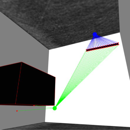
Sensor positioning in electrical cabinets: A company producing electrical components were producing sensors which shut off the power if an electrical arc appears in a cabinet. The sensors which detect such arcs have to be positioned within the cabinet, and they wanted to determine optimal sensor positions when the cabinets included obstacles.
Calibrating gyroscopes for side-mirror rotation: This company were producing a hardware/software solution for rotating the side mirror on large trucks, such that the mirror always faced the right way when the trucks were turning. Two gyroscopes were used for measuring the angle of rotation – but gyroscopes have a tendency to drift quite a lot. They wanted a way to reduce the amount of drift using accelerometer data.
Modelling water flow in a root-screening facility: A grass-producing company wanted to dynamically control water levels in a facility for testing root-depth. They wanted to use a set of valves and sensors to have a complex water saturation structure in the soil.
Algorithm optimisation for optimal robot accelerations: A company producing robots wanted to optimise one of their algorithm for moving robot arms. When a robot arm with many joints received a new instruction on where to move, it calculated an optimal way to turn the joints to follow a path there. Each joint has a maximum rotational torque, and their algorithm for determining how to rotate the joints while obeying torque constraints was too slow.
I worked on the first problem of optimally placing light sensitive sensors within an electrical cabinet. The problem we faced looks somewhat similar to the Art Gallery Problem, but the 3-dimensional cabinets make the problem quite a bit less trivial to solve. We developed and implemented algorithms which placed sensors optimally in 3d cabinets like the one shown below:
This was my fifth study group with industry, and it was an immense pleasure as always. There are in particular two things which I think ESGI makes very clear:
Real math is very hard: When studying a degree in mathematics, one rarely gets to work on real problems. Most of the “real” problems that is encountered throughout the years of studying are the nicest examples of real problems to be found, where they are often picked since they highlight some theory which perfectly solve the problem. In reality, many problems are either intractable, solvable by rather simple math or simply a test of ones skills in understanding the details of the asked problem.
Everybody have something to offer: What surprised me a lot at my first study group is that senior researchers and young students both have a lot to offer when it comes to solving industrial problems. The young students often have fresh perspectives on the problems and superior coding skills, where senior people have a load of experience with mathematical modelling. It is an amazing experience to throw away the normal hierarchies and work together; bachelor students, PhD students and professors.
For the blog post I have interviewed a number of the best users on Kaggle about their tips and tricks for winning Kaggle competitions. The post is a collection of the best of their answers together with some of my own experiences and tips for competitive machine learning.
This year, Copenhagen is hosting the EuroScience Open Forum conference which Europe’s largest, general science meeting. The conference includes – among other things – a programme of seminars, workshops and debates about science and technology, a Science in the City programme to engage with the general public and different exhibitions and events to promote science.
I was lucky to get a free ticket from DTU, which enables me to participate in the seminars, workshops and events at the conference.
Monday, June 23
On my first day of the conference, I participated in two talks, one titled: “Neuroenhancement: a true unfolding of man” and one titled: “The billion-dollar big brain projects: where are we going with our brains?“. The first talked about the potentials and risks of enhancing the human brain in general, and the second gave an outline of the visions and progress of the Human Brain Project and the new BRAIN Initiative.
The Sensible DTU Project which I am a part of, has a booth in The House of Future Technologies. In this booth, we showcase our research on social networks, human mobility and large scale data analysis. Additionally, we have developed a mobile app for the Science in the City programme which besides holding information about the conference, contains a competition. To participate in the competition, one needs to sign up with Facebook, and we then track the number of steps taken by each participant. The more steps you take, the more vouchers you get for the final lottery where you can win iPads and Fitbit bracelets. The data generated by the competition is to be used in a scientific study of exercise-related habits and motivation.
Talk titled: Neuroenhancement: a true unfolding of man.
Seth Grant from The University of Edinburgh talking about The Human Brain Project.
The billion-dollar big brain projects: where are we going with our brains?
Some of the nice facilities at Carlsberg.
One of the visualisations at our booth in The House of Future Technologies – together with some of our prices.
Tuesday, June 24
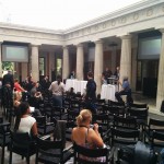
I started out the morning by attending a panel-debate about the future of Massive Open Online Courses (MOOC’s) in higher education. The panelists were
PatrickAebischer, the president of Ecole Polytechnique Fédérale de Lausanne (EPFL)
JohannesHeinlein, Director of Strategic Partnerships and Collaborations, edX
VolkerZimmermann, Member of the Board, IMC AG – IMC information multimedia
Ana Carla Pereira, Head of Unit, Directorate General Education and Culture, European Commission
It was pleasing to hear especially Patrick Aebischer express some very positive and ambitious goals and visions for the future of MOOC’s, both globally and in Europe.
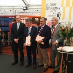
After the panel-debate, I attended the launch of a new popular science magazine: Technologist. The magazine is produced by the EuroTech Universities Alliance, which features The Technical University of Denmark, Technical University of Munich, Eindhoven University of Technology and Ecole Polytechnique Fédérale de Lausanne.
One of the events around the launch party, was an ice-cream stand, where the free ice-cream was spiced up with proteins artificially grown in labs. I got an ice-cream with “meat” grown from the muscle tissue of the Dutch king, and Kristina got a very politically-incorrect panda ice-cream!
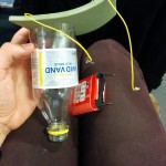
After lunch I participated in a session on how to teach engineering to kids. The session included a very inspiring talk from Ioannis N. Miaoulis, the President and Director of the Museum of Science in Boston. After his talk, the audience – in pairs – had to assemble a simple vacuum cleaner as a show-case of how to get engineering into the classroom.
Finally I participated in an extended session with the title: “Minding humans” together with one of my colleagues Camilla Birgitte Falk Jensen, which featured 4 very different talks on ranging from gender issues in research over art to social neuroscience.
Talk by Cordelia Fine on the delusions of gender – with perspectives to modern neuroscience.
A home-made vacuum cleaner, made by me and my side-partner to illustrate how to teach kids about engineering.
Talk on teaching engineering to kids by Ioannis N. Miaoulis, the president of The Museum of Science in Boston.
The 4 presidents of the universities in the EuroTech Universities Alliance.
Kristina Linde Hansen “enjoying” an ice-cream based on artificially grown meat cells from pandas.
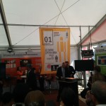
Launch of the new science magazine “Technologist”.
Hors d’oeuvres for the launch party.
Panel discussion on the future of MOOC’s in higher education.
Wednesday, June 25
One of the events at ESOF2014 was Picnic with the Prof, a chance for young researchers (as me) to meet and eat lunch with professors and professionals within science and research. I had the pleasure of eating lunch with Cédric Villani, a Fields medalist within partial differential equations and mathematical physics. Besides me and Cédric, the table featured a physicist from KU working on predicting the next ice age and 3 young researchers working with algebra, algebraic topology and topology (there was definitely a trend!). We talked about everything from millenium problems and Danish food to quantitative finance and the aftermath of winning a Fields medal.
After the lunch I attended a seminar titled “Should science always be open?” which featured 4 speakers each giving their personal angle on the questions. The seminar tackled both the publishing part of open access to research and questions about how to handle open access to data sets containing personal data. During the session, each table had a brainstorming session about the pros and cons of open access. Throughout the entire session, the speakers and their comments were drawn on a large sheet of paper.
Live drawing of the panel discussion and synergy workshop on open access, open data and open science.
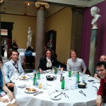
Lunch with Fields medalist Cédric Villani and 4 other young researchers.
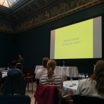
Session titled “Should science always be open?”.
Live drawing of the session on open access.
Conclusion
Participating in ESOF2014 has been a great experience. The conference was definitely not a traditional scientific conference, but rather a chance to look at science from a higher perspective. I met a lot of interesting and fascinating people (at least 4 people asked for my business card), heard some great talks and got a chance to present my own research to a number of people.
As most researchers and students of technical degrees, I have used LaTeX for a long time. One of the newer LaTeX-related innovations is the possibility to use online editors to manage your LaTeX projects. Two of the most prominent sites for this are ShareLaTeX and writeLaTeX, which are very similar. Recently I was asked about the difference between the two after I had recommended ShareLaTeX which I was using myself, and had no luck finding a good overview of the differences between the two services. Consequently I have tried to compile a description of the differences.
Feature
ShareLaTeX
writeLaTeX
Real time collaboration
Yes
Yes
Change history
Yes1
Yes
Max # users for free
2
Unlimited
Max # users paid
Unlimited2
Unlimited2
Open source
Yes
No3
Sync to Dropbox
Yes4
Yes4
Templates
Yes
Yes
Mobile device support
No5
Yes
Real time preview
No
Yes
Spell-check
Yes
Yes
Auto-complete LaTeX
Yes6
Yes6
Requires the 15$/month plan
ShareLaTeX gives you 11 users for 15$/month and unlimited for 30$/month
At least not as far as I could see
Requires paid plans: Minimum 15$/month for ShareLaTeX and 7$/month for writeLaTeX
I tried on my Android phone, and while it might work on larger screens, using a phone does not work.
The auto-complete in ShareLaTeX is more advanced. For example: If you write begin{tabular}, ShareLaTeX will give you the end{tabular} and insert the required parameters for the begin-command. writeLaTeX will only auto-complete your begin{tabular} line (backslashes omitted due to MathJax issues)
Conclusions
There is no clear winner between the two services which are both really nice! The paid plans for writeLaTeX are a bit more affordable, and it gives a few more free features. There is a student discount plan for ShareLaTeX which makes the plans quite similar in price. Personally I like the interface in ShareLaTeX more, and the compiled pdf-files shown in the browser looks better in ShareLaTeX (you have the option to choose between different pdf-viewers).
If I have missed a feature or in general made any mistakes in my comparison, please write a comment and I will fix whatever mistakes I have made.
Recently the competition titled Galaxy Zoo – The Galaxy Challenge ended on the Kaggle.com platform. I participated in this competition (as part of my thesis) and ended up placing in the top 10% with a 28th place of out 329 participants. In this post I will give a brief description of Kaggle competitions, the Galaxy Zoo problem and describe my approach to solving the problem together with lessons learned from the other participants.
Kaggle Competitions
Kaggle provides an amazing platform for running competitions in predictive data analysis. At all times, a number of competitions is running where the participants are asked to predict some variable based on provided data. The competitions can be about predicting product sales for large companies, optimising flight traffic, determining if people are psychopaths from their tweets or classifying galaxies from deep space image data.
The participants are provided with a data set of with a description of the variables, a target variable to predict and an error-measure to optimise. The data set is split into three parts – a training set, a public test set and a private test set. For the training set, the participants are given the value of the target variable, while this is not provided for the test sets.
The participants submit predictions for the target value on the test set (both public and private – since it is not public how these two sets are split) and get an error back computed on the public part of the test set. The participants are then ranked by their public test set error and these results are shown on a public leaderboard.
When the competition is over, the scores on the private test set is made public and those with lowest scores on the private test set will take home the money!
The Galaxy Zoo Problem
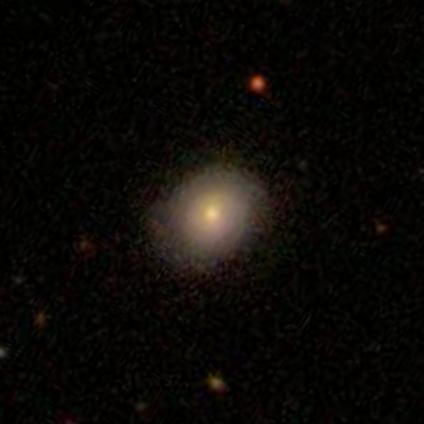
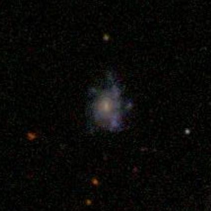
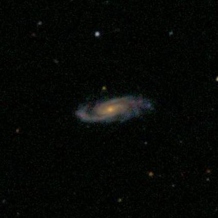
The problem of this competition was to classify galaxies based on image data from a deep space telescope. The data given was a set of 141,553 image (61,578 in the training set and 79,975 in the test set) which looks like this:
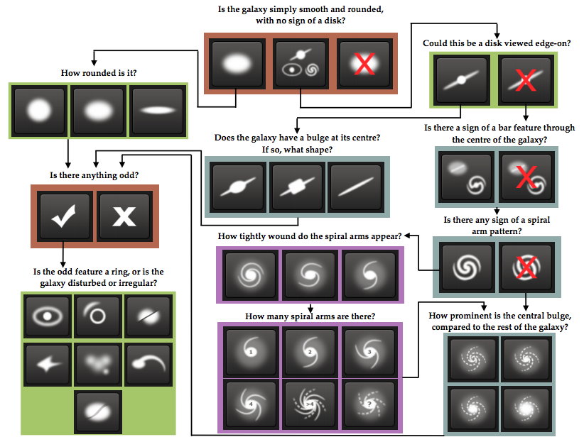
For each galaxy, a number of human users have been asked a series of questions used to classify the galaxy. Which questions are asked depends on the answers to previous questions, so the possible questions can be described by a decision tree. This decision tree looks like this:
The task of classifying galaxies is not easy, and often the human classifiers disagree on the questions in the decision tree. To quantify these disagreements, we are given data on how the users distribute on the possible answers. The task is to predict how the users of Galaxy Zoo distribute on the possible answers to each question. Say that for a specific galaxy, 20% answers that the galaxy is “smooth”, 60% answers it is “features or disk” and the last 20% answers that it is “star or artefact”, then the first three values in the output for that galaxy will be
$$\left[ 0.2, 0.6, 0.2 \right].$$
To put priority on the most important questions in the decision tree which determines the overall structure of the galaxy (the questions in the top of the tree), the later questions are down-weighted. Continuing the example above, look at the 60% who answered “features or disk”. These 60% now go to Question 2, and say that 70% answers “yes” and 30% answers “no”. Then the next two outputs for this galaxy will be
since we distribute the 60% answering “features or disk” on the first question into two parts of relative size 70% and 30%. Additionally, the answers to Question 6 have been normalised to sum to 1.
The scoring method in this competition was Root Mean Squared Error defined as:
where \(t_{ij}\) is the actual value for sample \(i\), feature \(j\) and where \(p_{ij}\) is the predicted value for sample \(i\), feature \(j\).
Our Approach
I started out by making a simple benchmark submission. For each of the 37 outputs, I computed the average value in the training data, obtaining a vector of 37 elements. Submitting this vector as the prediction for each image in the test set gave a RMSE score of 0.16503 (I will emphasise scores on the leaderboard with bold in the rest of this post).
To make it easier to extract features and learn from the image data, I pre-processed the raw input images. The code for pre-processing is written in Python, using the scikit-image library. The pre-processing consisted of the following steps:
Threshold the image to black and white using Otsu’s method – which is a method for automatically inferring the optimal thresholding level.
Use a morphological closing operation with a square of size \(3 \times 3\) as kernel.
Remove all objects connected to the image border.
Remove all connected components for which the bounding box is less than 256 in area.
Find the connected component \(C\) closest to the center of the image.
Rescale the bounding box of \(C\) to be a square by expanding either the width or the height and add 15 pixels on each side.
In the original image, take out the portion contained in the expanded version of \(C\).
Rescale the image to \(64 \times 64\) pixels.
Using this pre-processing, the images now looked like this:
Next I trained a convolutional neural network on the training data using the MATLAB implementation by Rasmus Palm. The first layer in the network was a convolutional layer with 6 output maps and a kernel size of 21. The second layer was an average pooling layer with a scaling factor of 2. The third layer was a convolutional layer with 12 output maps and a kernel size of 5. The fourth layer was an average pooling layer with a scaling factor of 2. The final layer was a fully-connected layer with 37 output neurons. All layers used the sigmoid activation function. To avoid overfitting, I trained the network with a validation set of 5,000 images. If the error on the validation does not lower over 5 epochs in a row, the training was stopped and the network with the minimum validation error was saved.
Training this network architecture on 10,000 of the 61,578 training images, I obtained a leaderboard score of 0.13172. Training the same architecture on 30,000 images from the training data, I obtained a leaderboard score of 0.12056.
One way to get more performance out of a deep neural network, is to generate more training data using invariances in the data. One example of such an invariance in the galaxy data is rotational invariance since a galaxy can appear in an arbitrary rotation. Other possible invariances are translation and scale, but since the galaxies after pre-processing do not have much space on either side (they tend to fill out the image), this is not as easy to exploit (although other teams actually had success with this). I trained the same network as before on 55,000 of the training images , where each image was also added after a rotation of 90 degrees, giving a total number of 110,000 training samples. Training the network took 80 epochs and a total of 53 hours.
When doing predictions on the test set, I sent each test image through the network four times, rotated 0, 90, 180 and 270 degrees, averaging the outputs. The validation error on the network was 0.1113. Feeding 4 different rotations through the network and averaging them gave a validation score of 0.1082. Finally, post-processing the output to obey the constraints of the decision tree reduced the validation error to 0.1077. On the leaderboard this gave a score of 0.10884.
Next I tried a different architecture for the network:
Convolutional layer with 6 output maps and kernels of size \(5 \times 5\)
Factor 2 average pooling
Convolutional layer with 12 output maps and kernels of size \(5 \times 5\)
Factor 2 average pooling
Convolutional layer with 24 output maps and kernels of size \(4 \times 4\)
Factor 2 average pooling
Fully connected layer
This network reached a validation error of 0.1065 after 49 epochs (around 60 hours of training time). By inputting the test set with four different rotations and post-processing the output, this gave a leaderboard score of 0.10449.
I then tried the following architecture:
Convolutional layer with 8 output maps and kernels of size \(9 \times 9\)
Factor 2 average pooling
Convolutional layer with 16 output maps and kernels of size \(5 \times 5\)
Factor 2 average pooling
Convolutional layer with 32 output maps and kernels of size \(5 \times 5\)
Factor 2 average pooling
Convolutional layer with 64 output maps and kernels of size \(4 \times 4\)
Fully connected layer
This network reached a validation error of 0.0980 after 76 epochs (around 160 hours). On the leaderboard this network obtained a score of 0.09655 (with post-processing and rotated test images).
Finally, I trained a network with the same architecture as above, but with colour images (done by inputting each of the three colour channels to the network). This obtained a leaderboard score of 0.09322.
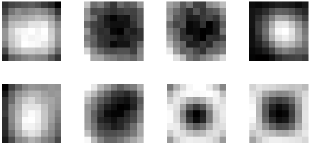
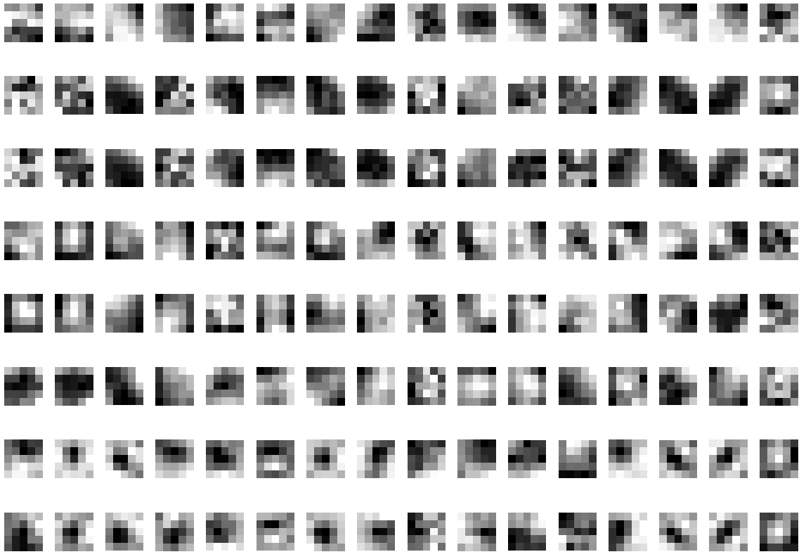
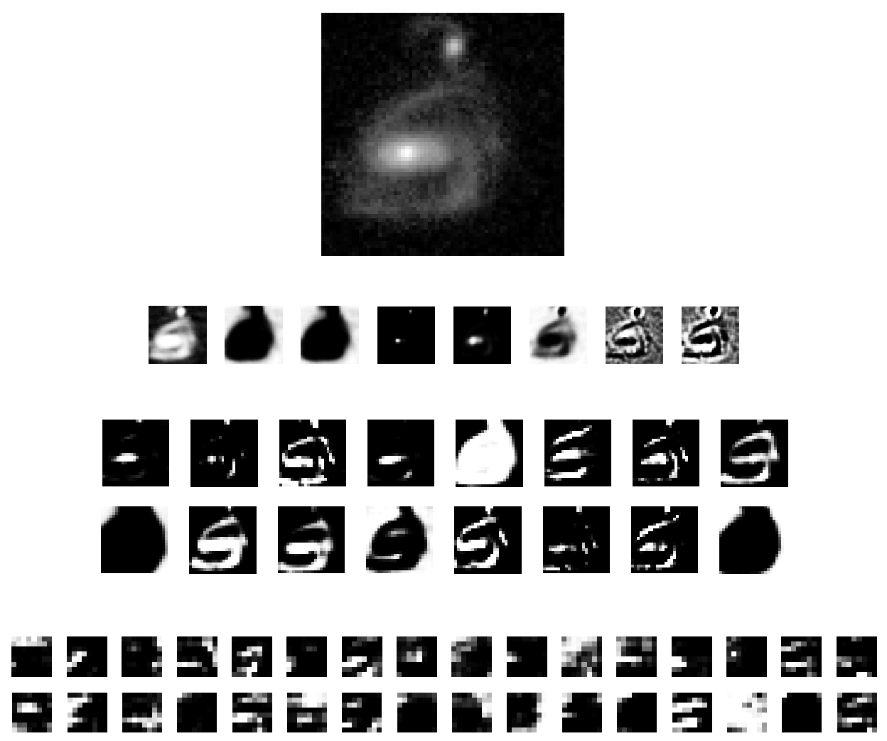
To understand how images are processed by the networks I have plotted some of the learnt kernels and visualisations of how an image is propagated through the network. The visualisations are from the network obtaining a leaderboard score of 0.09655.
The 8 learnt kernels in the first convolutional layer.The 16 learnt kernels in the second convolutional layer. Note that each of these 16 kernels is 3-dimensional and consequently each column of this figure corresponds to one kernel.
A visualisation of how an image is propagated through the network. On the top is the original image which is input into the network. In the next layer the first 8 kernels have been applied, in the next layer the next 16 kernels and so forth.
By looking at the image being propagated through the first convolutional layer we can somewhat rationalise what the kernels are doing: The fourth and firth kernel are detecting the center of the galaxy, the second and third are extracting a rough outline of the galaxy and the rest are extracting more a detailed shape outline.
Results and Lessons Learned
When the private leaderboard was revealed, I finished on a 28th place with a total of 329 participants.
Normally, it is a good idea to start with simple models and iterate quickly, but in this competition I went almost directly to convolutional neural networks. There are multiple reasons for this: The first reason is that dataset is rather large (more than 50,000 data samples). The second reason is that the data has obvious invariances (translation and rotation) which can be used to generate even more data (even though I did not use translation). Finally, most recent literature on image recognition points to convolutional nets as the best possible approach [Ciresan et al., 2012].
One significant issue was the speed of MATLAB implementation. When training the final convolutional nets the training time approached three weeks per network. In principle there was no limit to amount of data that could be generated, and there were multiple ways to make the networks more complex. When training very complex models like convolutional neural networks, the efficiency of the implementation can be the deciding factor.
Another short-coming of my approach was that I was not predicting exactly the correct thing. Regarding the error-measure I was doing the correct thing by optimising mean squared error for the net, but when I was training the network I treated the problem as a regression problem instead of the multi-class classification problem it really is. The problem with this is that the output is actually limited by 11 constraints which the networks were not utilising (the answer-proportions for the 11 different questions in the decision tree must sum to specific values). A better way to handle this problem is to construct a network for multi-class classification using a number of soft-max units, and to derive a correct loss-function for the network which incorporates the constraints of the decision tree directly.
Another trick which some of the top participants talked about after the competition was the use of polar coordinates for learning rotationally invariant features (see the really good write-up from the winner sedielem). This is a really interesting idea which I will be sure to look into if/when rotationally invariant image problems appear again.