Recently the competition titled Galaxy Zoo – The Galaxy Challenge ended on the Kaggle.com platform. I participated in this competition (as part of my thesis) and ended up placing in the top 10% with a 28th place of out 329 participants. In this post I will give a brief description of Kaggle competitions, the Galaxy Zoo problem and describe my approach to solving the problem together with lessons learned from the other participants.
Kaggle Competitions
Kaggle provides an amazing platform for running competitions in predictive data analysis. At all times, a number of competitions is running where the participants are asked to predict some variable based on provided data. The competitions can be about predicting product sales for large companies, optimising flight traffic, determining if people are psychopaths from their tweets or classifying galaxies from deep space image data.
The participants are provided with a data set of with a description of the variables, a target variable to predict and an error-measure to optimise. The data set is split into three parts – a training set, a public test set and a private test set. For the training set, the participants are given the value of the target variable, while this is not provided for the test sets.
The participants submit predictions for the target value on the test set (both public and private – since it is not public how these two sets are split) and get an error back computed on the public part of the test set. The participants are then ranked by their public test set error and these results are shown on a public leaderboard.
When the competition is over, the scores on the private test set is made public and those with lowest scores on the private test set will take home the money!
The Galaxy Zoo Problem
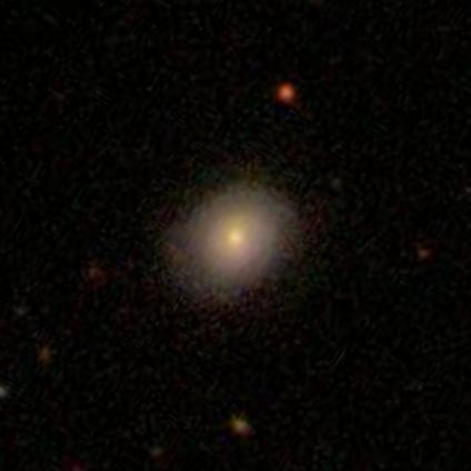
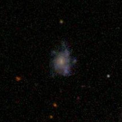
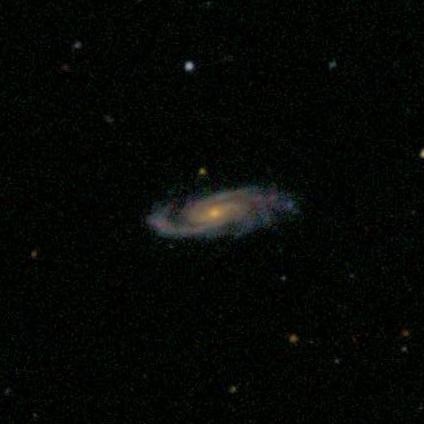
The problem of this competition was to classify galaxies based on image data from a deep space telescope. The data given was a set of 141,553 image (61,578 in the training set and 79,975 in the test set) which looks like this:
For each galaxy, a number of human users have been asked a series of questions used to classify the galaxy. Which questions are asked depends on the answers to previous questions, so the possible questions can be described by a decision tree. This decision tree looks like this:
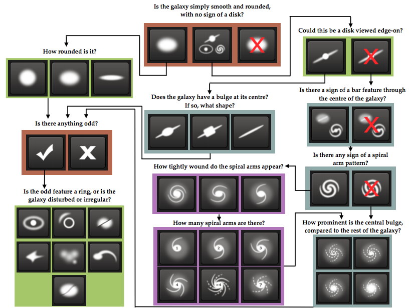
The task of classifying galaxies is not easy, and often the human classifiers disagree on the questions in the decision tree. To quantify these disagreements, we are given data on how the users distribute on the possible answers. The task is to predict how the users of Galaxy Zoo distribute on the possible answers to each question. Say that for a specific galaxy, 20% answers that the galaxy is “smooth”, 60% answers it is “features or disk” and the last 20% answers that it is “star or artefact”, then the first three values in the output for that galaxy will be
$$\left[ 0.2, 0.6, 0.2 \right].$$
To put priority on the most important questions in the decision tree which determines the overall structure of the galaxy (the questions in the top of the tree), the later questions are down-weighted. Continuing the example above, look at the 60% who answered “features or disk”. These 60% now go to Question 2, and say that 70% answers “yes” and 30% answers “no”. Then the next two outputs for this galaxy will be
$$\left[0.6 \times 0.7, 0.6 \times 0.3\right] = \left[0.42, 0.18\right],$$
since we distribute the 60% answering “features or disk” on the first question into two parts of relative size 70% and 30%. Additionally, the answers to Question 6 have been normalised to sum to 1.
The scoring method in this competition was Root Mean Squared Error defined as:
$$\text{RMSE} = \sqrt{\frac{1}{37N} \sum_{i=1}^N \sum_{j=1}^{37}(t_{ij}-p_{ij})^2},$$
where \(t_{ij}\) is the actual value for sample \(i\), feature \(j\) and where \(p_{ij}\) is the predicted value for sample \(i\), feature \(j\).
Our Approach
I started out by making a simple benchmark submission. For each of the 37 outputs, I computed the average value in the training data, obtaining a vector of 37 elements. Submitting this vector as the prediction for each image in the test set gave a RMSE score of 0.16503 (I will emphasise scores on the leaderboard with bold in the rest of this post).
To make it easier to extract features and learn from the image data, I pre-processed the raw input images. The code for pre-processing is written in Python, using the scikit-image library. The pre-processing consisted of the following steps:
- Threshold the image to black and white using Otsu’s method – which is a method for automatically inferring the optimal thresholding level.
- Use a morphological closing operation with a square of size \(3 \times 3\) as kernel.
- Remove all objects connected to the image border.
- Remove all connected components for which the bounding box is less than 256 in area.
- Find the connected component \(C\) closest to the center of the image.
- Rescale the bounding box of \(C\) to be a square by expanding either the width or the height and add 15 pixels on each side.
- In the original image, take out the portion contained in the expanded version of \(C\).
- Rescale the image to \(64 \times 64\) pixels.
Using this pre-processing, the images now looked like this:


Next I trained a convolutional neural network on the training data using the MATLAB implementation by Rasmus Palm. The first layer in the network was a convolutional layer with 6 output maps and a kernel size of 21. The second layer was an average pooling layer with a scaling factor of 2. The third layer was a convolutional layer with 12 output maps and a kernel size of 5. The fourth layer was an average pooling layer with a scaling factor of 2. The final layer was a fully-connected layer with 37 output neurons. All layers used the sigmoid activation function. To avoid overfitting, I trained the network with a validation set of 5,000 images. If the error on the validation does not lower over 5 epochs in a row, the training was stopped and the network with the minimum validation error was saved.
Training this network architecture on 10,000 of the 61,578 training images, I obtained a leaderboard score of 0.13172. Training the same architecture on 30,000 images from the training data, I obtained a leaderboard score of 0.12056.
One way to get more performance out of a deep neural network, is to generate more training data using invariances in the data. One example of such an invariance in the galaxy data is rotational invariance since a galaxy can appear in an arbitrary rotation. Other possible invariances are translation and scale, but since the galaxies after pre-processing do not have much space on either side (they tend to fill out the image), this is not as easy to exploit (although other teams actually had success with this). I trained the same network as before on 55,000 of the training images , where each image was also added after a rotation of 90 degrees, giving a total number of 110,000 training samples. Training the network took 80 epochs and a total of 53 hours.
When doing predictions on the test set, I sent each test image through the network four times, rotated 0, 90, 180 and 270 degrees, averaging the outputs. The validation error on the network was 0.1113. Feeding 4 different rotations through the network and averaging them gave a validation score of 0.1082. Finally, post-processing the output to obey the constraints of the decision tree reduced the validation error to 0.1077. On the leaderboard this gave a score of 0.10884.
Next I tried a different architecture for the network:
- Convolutional layer with 6 output maps and kernels of size \(5 \times 5\)
- Factor 2 average pooling
- Convolutional layer with 12 output maps and kernels of size \(5 \times 5\)
- Factor 2 average pooling
- Convolutional layer with 24 output maps and kernels of size \(4 \times 4\)
- Factor 2 average pooling
- Fully connected layer
This network reached a validation error of 0.1065 after 49 epochs (around 60 hours of training time). By inputting the test set with four different rotations and post-processing the output, this gave a leaderboard score of 0.10449.
I then tried the following architecture:
- Convolutional layer with 8 output maps and kernels of size \(9 \times 9\)
- Factor 2 average pooling
- Convolutional layer with 16 output maps and kernels of size \(5 \times 5\)
- Factor 2 average pooling
- Convolutional layer with 32 output maps and kernels of size \(5 \times 5\)
- Factor 2 average pooling
- Convolutional layer with 64 output maps and kernels of size \(4 \times 4\)
- Fully connected layer
This network reached a validation error of 0.0980 after 76 epochs (around 160 hours). On the leaderboard this network obtained a score of 0.09655 (with post-processing and rotated test images).
Finally, I trained a network with the same architecture as above, but with colour images (done by inputting each of the three colour channels to the network). This obtained a leaderboard score of 0.09322.
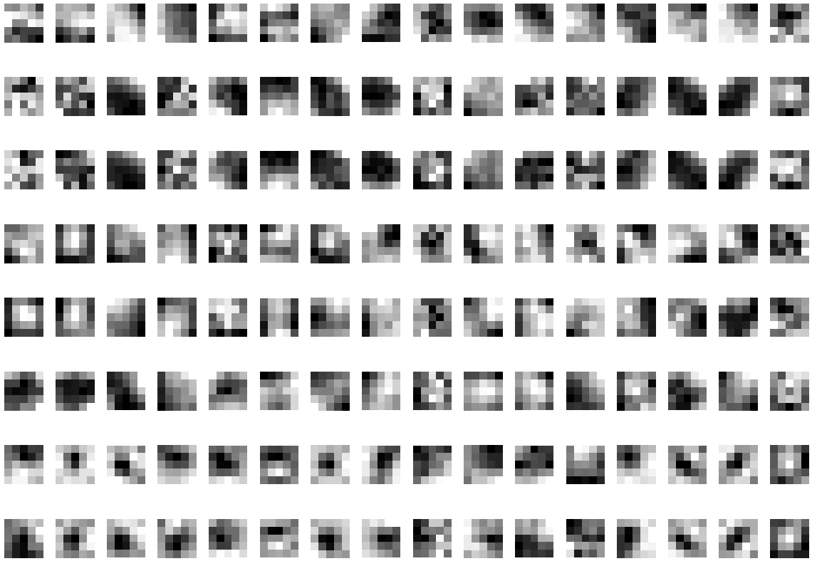
To understand how images are processed by the networks I have plotted some of the learnt kernels and visualisations of how an image is propagated through the network. The visualisations are from the network obtaining a leaderboard score of 0.09655.
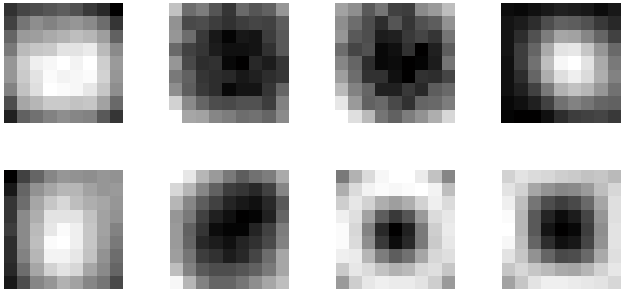
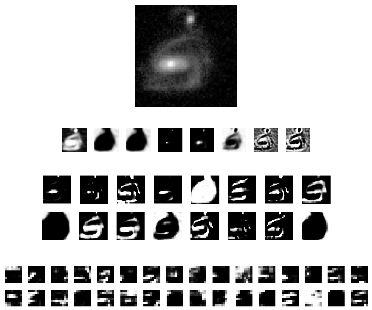
By looking at the image being propagated through the first convolutional layer we can somewhat rationalise what the kernels are doing: The fourth and firth kernel are detecting the center of the galaxy, the second and third are extracting a rough outline of the galaxy and the rest are extracting more a detailed shape outline.
Results and Lessons Learned
When the private leaderboard was revealed, I finished on a 28th place with a total of 329 participants.
Normally, it is a good idea to start with simple models and iterate quickly, but in this competition I went almost directly to convolutional neural networks. There are multiple reasons for this: The first reason is that dataset is rather large (more than 50,000 data samples). The second reason is that the data has obvious invariances (translation and rotation) which can be used to generate even more data (even though I did not use translation). Finally, most recent literature on image recognition points to convolutional nets as the best possible approach [Ciresan et al., 2012].
One significant issue was the speed of MATLAB implementation. When training the final convolutional nets the training time approached three weeks per network. In principle there was no limit to amount of data that could be generated, and there were multiple ways to make the networks more complex. When training very complex models like convolutional neural networks, the efficiency of the implementation can be the deciding factor.
Another short-coming of my approach was that I was not predicting exactly the correct thing. Regarding the error-measure I was doing the correct thing by optimising mean squared error for the net, but when I was training the network I treated the problem as a regression problem instead of the multi-class classification problem it really is. The problem with this is that the output is actually limited by 11 constraints which the networks were not utilising (the answer-proportions for the 11 different questions in the decision tree must sum to specific values). A better way to handle this problem is to construct a network for multi-class classification using a number of soft-max units, and to derive a correct loss-function for the network which incorporates the constraints of the decision tree directly.
Another trick which some of the top participants talked about after the competition was the use of polar coordinates for learning rotationally invariant features (see the really good write-up from the winner sedielem). This is a really interesting idea which I will be sure to look into if/when rotationally invariant image problems appear again.